EasyPPO: Stabilizing the Critic Is Key

Six panels compare EasyPPO, PPO, PPO with actor-only filtering, HL-Gauss PPO, and VAPO. Columns are FrontierCS, AIME, and Search-R1. Training curves are on top, validation below. EasyPPO preserves its gains while every baseline collapses in at least one task. — **EasyPPO achieves the best validation scores and remains stable across all three tasks.** Training above, validation below; one run per method and task.

The idea in a minute

PPO^[1] uses a critic to estimate how much reward a response is likely to earn. The actor uses that estimate to decide which responses to reinforce. If critic learning becomes unstable, the actor can lose a useful training signal.

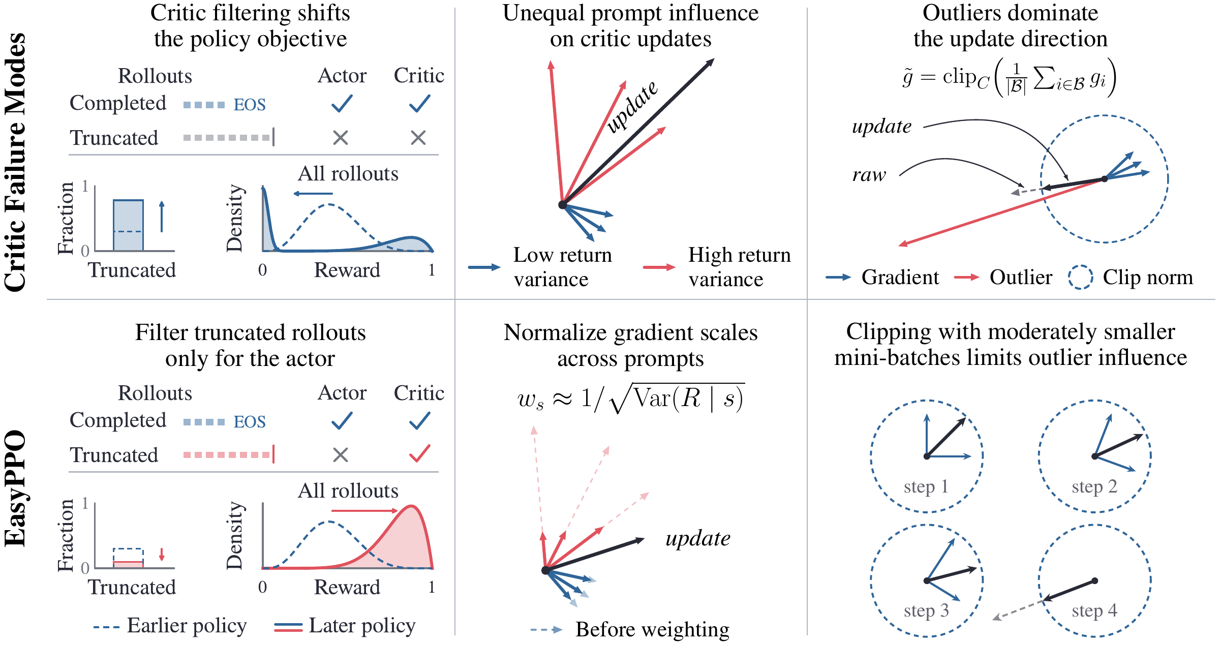
Keep the critic’s training data complete. Filter unfinished responses from actor updates, but keep them when training the critic.

Balance the noise across prompts. Weight each prompt’s critic loss by the inverse standard deviation of its sampled returns.

Limit how far outliers reach. Use moderately smaller critic mini-batches, with gradient clipping at each update.

You can keep the standard PPO actor update or use your preferred actor-side improvements.

Overlong filtering can shift the policy objective

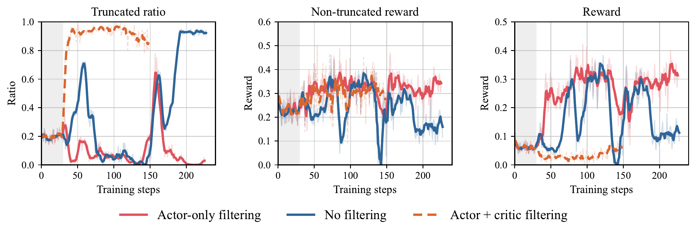
A response that hits the length limit may receive a low reward simply because it never finished. Filtering these responses from actor updates is common. In PPO, it is tempting to remove them from critic training too.

But then the critic only sees responses that finish. It learns their average reward instead of the average over all responses. Our analysis shows that, in an idealized accurate-critic setting, filtering both networks changes the policy objective to reward conditioned on completion. That score can improve even as more responses hit the length limit.

FrontierCS filtering comparison: joint actor-and-critic filtering leads to high truncation; completed-response rewards can rise while overall rewards remain low. Actor-only filtering improves overall reward but still shows instability. — **Reward among completed responses tells only part of the story.** FrontierCS, with a 32,768-token response limit.

The change: filter truncated responses only from actor updates. Keep every response for critic learning, so the critic can learn about unfinished responses too. This helps, but does not by itself prevent collapse.

A noisier prompt should not dominate the update

The same prompt can produce responses with very different rewards. Some prompts have consistent returns; others vary widely, especially in continuous-score coding tasks. We call this variation return noise.

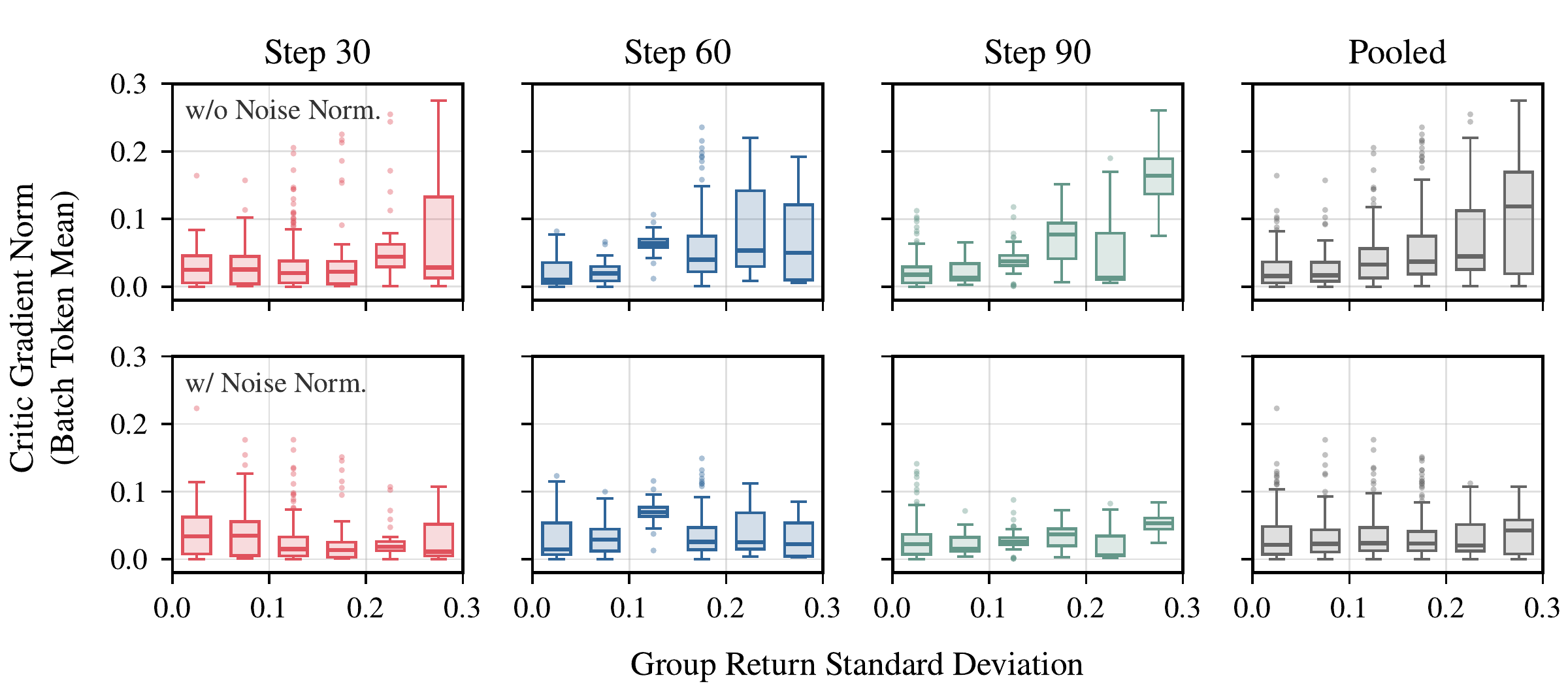
The critic tries to predict the mean return, but trains on individual samples. Even when its prediction is accurate, a noisy sample can produce a large gradient. For squared-error loss and a linear value head, the expected squared gradient contains both prediction error and return variance:

Expected squared critic gradient given s equals the squared feature norm times squared prediction error plus conditional return variance.

Here, s is a token prefix, R is its sampled return, and the value head predicts V(s) = W^⊤h(s). As predictions improve, the noise term can dominate this second moment. Prompts with more variable returns can therefore have disproportionate influence on finite-batch updates.

Normalize the noise, keep the prediction target

Noise-normalized critic regression divides the critic loss by the return standard deviation. If we knew the true conditional standard deviation at every prefix, setting w(s) to its inverse would give:

With the ideal weight, one over the conditional return standard deviation, the gradient second moment equals the squared feature norm times normalized squared prediction error plus one. The return-noise term is constant.

The return-noise term is now one. Apart from the feature norm, the second moment reflects the normalized prediction error. Positive population weights preserve the optimal mean prediction while removing return-noise scale as a source of imbalance.

From rollout groups to a weighted loss

In practice, we estimate one standard deviation per prompt from its group of n sampled returns, including truncated responses. We reuse that estimate at every token in the response. Writing R̄_s for the group’s mean return and ℬ for the prompt batch, we compute:

For each prompt s, estimate the return standard deviation using the mean squared deviation of its n sampled returns, with divisor n. Set w(s) to one over max of estimated standard deviation and epsilon, then divide by the average of these inverse standard deviations over prompts in batch B.

The floor ε prevents near-zero variance from producing an enormous weight. Dividing by the batch average keeps the prompt weights at mean one, so normalization does not arbitrarily rescale the whole loss.

Weighted critic loss equals one over twice the batch total valid-token count, times the sum over responses i of prompt weight w(s_i) times the sum over tokens t of squared prediction error, V(s_i,t) minus R_i.

Response i has prompt s_i, return R_i, and T_i valid tokens; s_i,t is its prefix at token t. The denominator averages over the batch’s valid tokens. Estimating weights from the same returns can introduce bias, but works well in our experiments.

A floor tied to reward range and group size

For discrete rewards with range Δ, consider a group with one maximum return and n − 1 minimum returns. We choose the floor to be approximately half this reference group’s standard deviation:

A reference group with one maximum return and n minus one minimum returns has standard deviation Delta times the square root of (1/n)(1 minus 1/n). Choose epsilon = Delta divided by twice square root n, approximately half the reference standard deviation.

With inverse-STD weighting, a group whose returns are all identical then gets about twice the weight of the reference group. For n = 16, this gives ε = 0.125 for Search-R1’s [0, 1] rewards and ε = 0.25 for AIME’s [−1, 1] rewards. FrontierCS has continuous rewards; we retain ε = 0.075 from our initial experiments.

The same pattern appears in actual gradients

As the critic learns, return noise accounts for more of the gradient scale. In the offline comparison below, the dependence on return variability becomes stronger at later checkpoints. Applying the weights largely flattens it, although some individual outliers remain. Each response contributes its summed token gradients divided by the batch’s total token count.

Box plots at training steps 30, 60, and 90 and pooled across those steps. Before normalization, prompts with higher return standard deviations tend to have larger gradient contributions. After normalization this relationship is much weaker. — **Normalization reduces the imbalance.** FrontierCS checkpoints 30, 60, and 90; unweighted gradients above, weighted below.

What changes: normalization makes gradient contributions more balanced across prompts. We handle the remaining outliers through the size of each critic mini-batch.

Smaller mini-batches make clipping more local

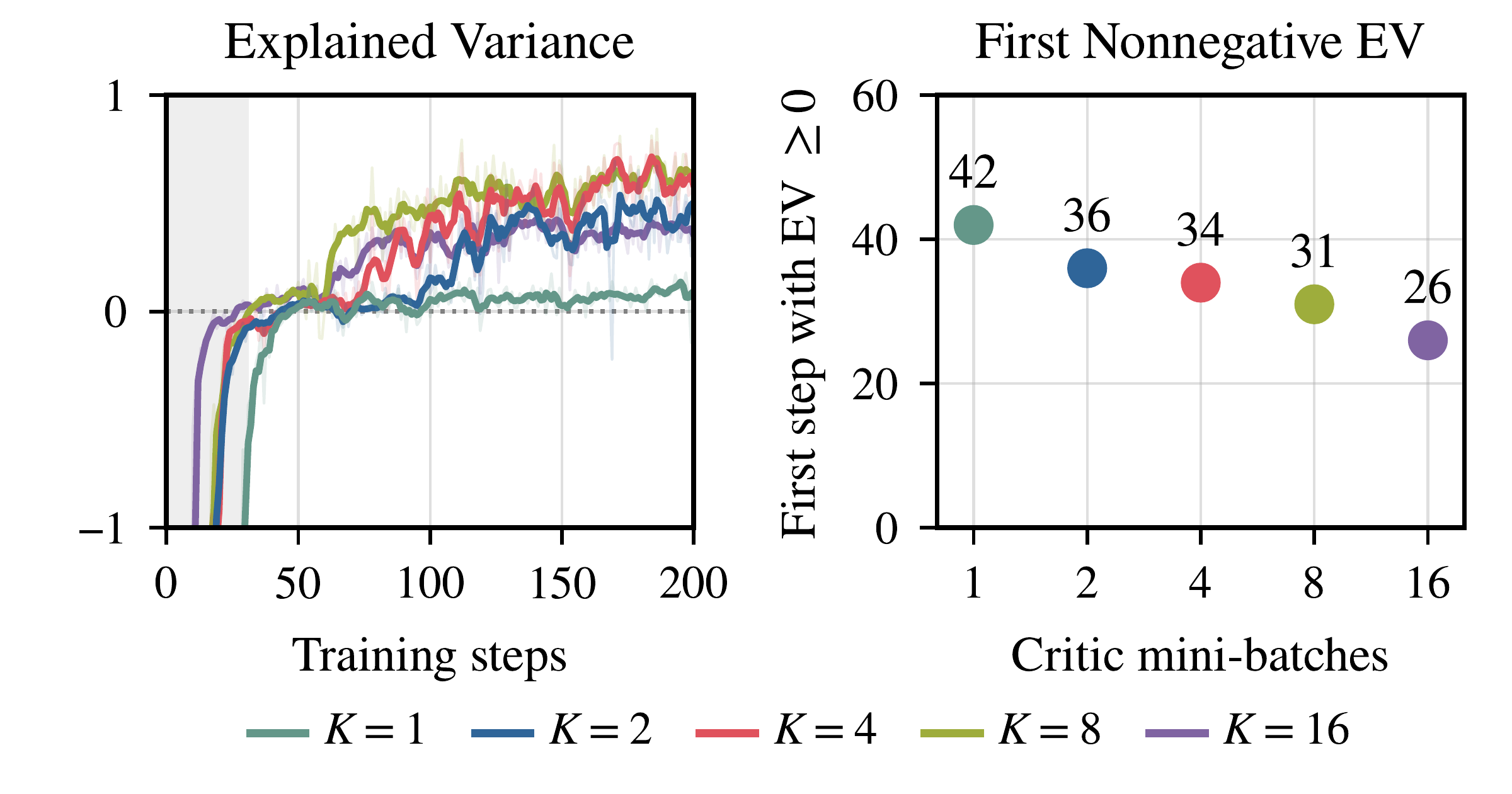
Gradient clipping rescales an entire mini-batch gradient when its norm is too large. If one outlier dominates a large mini-batch, clipping scales down everyone’s contribution together. Splitting the batch means fewer responses are affected by that outlier.

There is a trade-off: smaller mini-batches also average out less return noise. Our idealized analysis captures these opposing trends. The bound on a single outlier’s influence grows with mini-batch size, while the gradient variance falls with it. Smaller is therefore not always better.

FrontierCS critic explained variance for 1, 2, 4, 8, and 16 mini-batches. More splits reach nonnegative explained variance sooner, but four and eight achieve higher explained variance later in training. — **Finer splits help early; averaging matters later.** Fixed rollout batch, with learning rate scaled as $1 divided by the square root of K$ for K mini-batches.^[2]

Our choice: four critic mini-batches per rollout batch, clipping each averaged mini-batch gradient before its optimizer step. The next mini-batch uses the updated critic.

Higher scores, without late training collapse

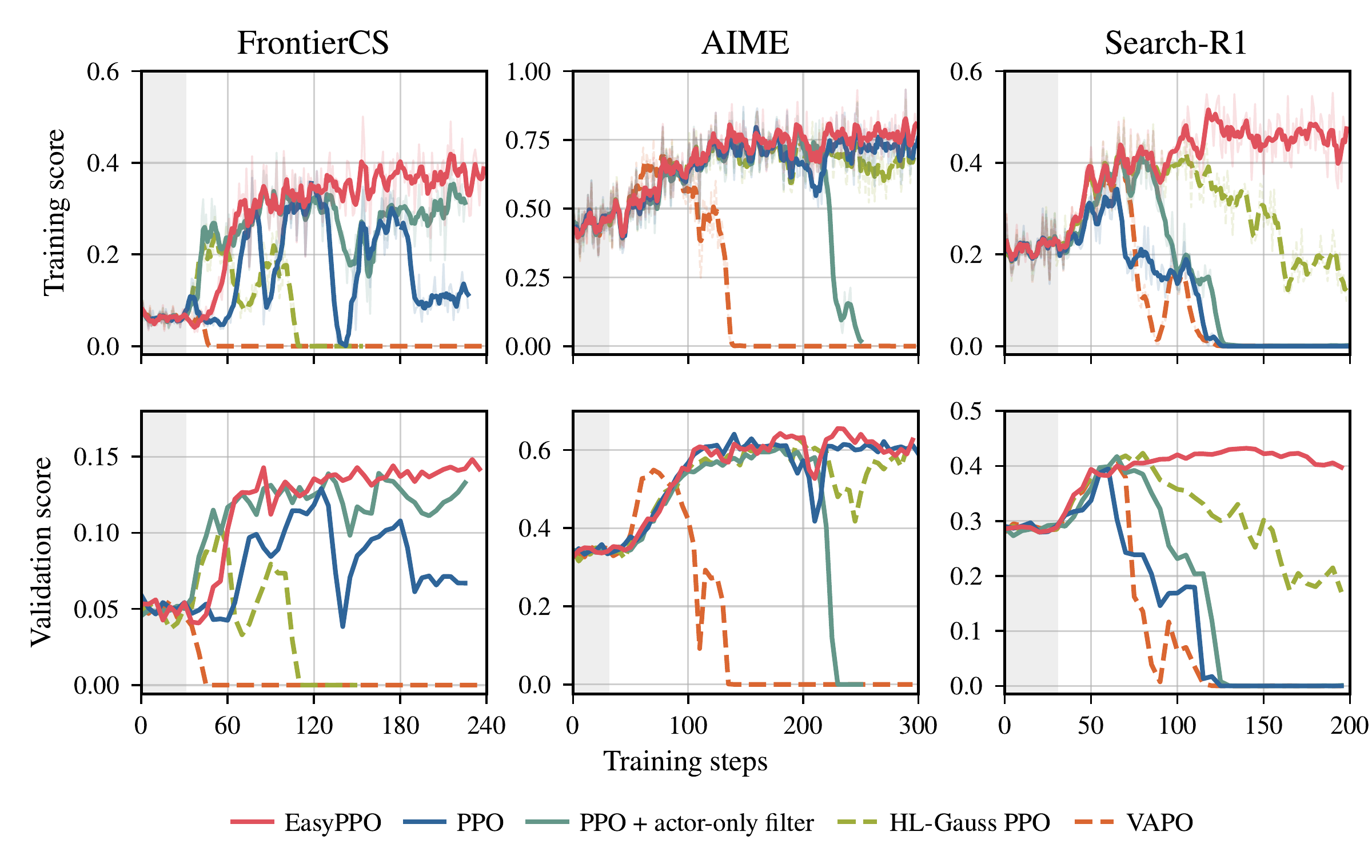
We test continuous-score coding on FrontierCS^[3], single-turn math on AIME24, and multi-turn search on Search-R1^[4]. EasyPPO achieves the highest best-checkpoint validation score on all three. Over the evaluated training horizons, it is also the only compared method that stays stable across all three tasks.

We compare against PPO, PPO + actor-only filtering, HL-Gauss PPO^[5], and VAPO^[6], omitting VAPO’s auxiliary positive-example language-modeling loss.

All methods train strictly on-policy in verl^[7], with 30 critic warmup steps. For FrontierCS, we initialize Qwen3.5-9B^[8] with SFT on FrontierSmith^[9] trajectories; AIME and Search-R1 use Qwen3.5-9B-Base.

Best validation scores (0–100)
Method	FrontierCS	AIME24	Search-R1
PPO	12.90	64.06	39.48
PPO + actor-only filtering	13.91	60.73	41.74
HL-Gauss PPO	10.43	63.13	42.33
VAPO	5.58	54.90	40.36
EasyPPO	14.82	65.52	43.22

Comparing each method’s best checkpoint, EasyPPO improves on PPO by 14.89% on FrontierCS, 2.28% on AIME24, and 9.47% on Search-R1.

A steadier critic accompanies steadier training

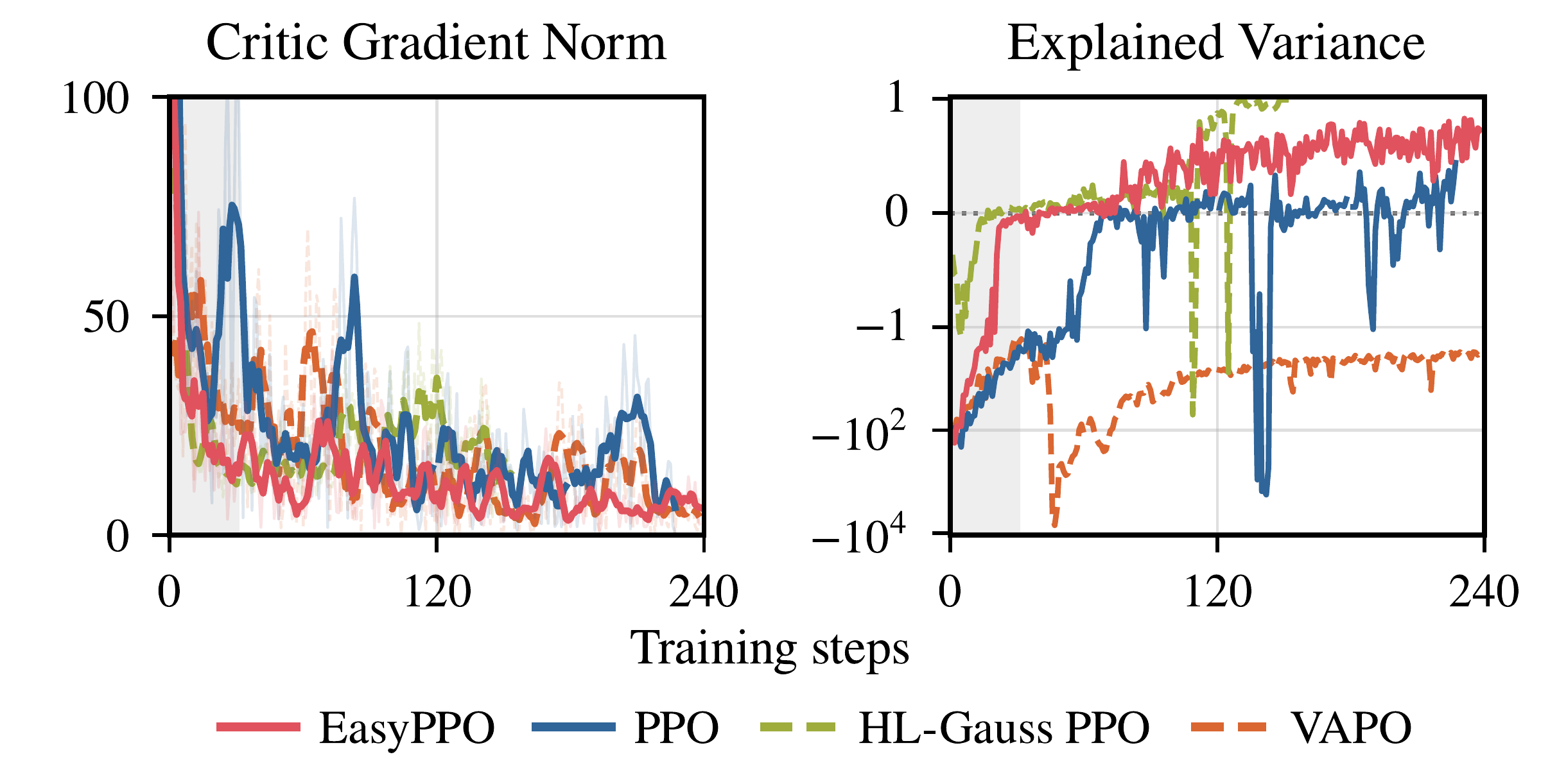
On FrontierCS, EasyPPO’s critic gradient norm declines after warmup, and its explained variance improves smoothly. The other methods show larger swings. High explained variance alone is not enough: HL-Gauss reaches nearly one after its actor has already collapsed, when predicting the consistently low return becomes easy.

FrontierCS critic gradient norm before clipping and explained variance. EasyPPO's gradients settle and its explained variance rises steadily, while the baseline curves fluctuate sharply. — **Stable critic learning accompanies sustained reward gains.** Gradient norms are measured before clipping.

Normalization creates room for smaller mini-batches

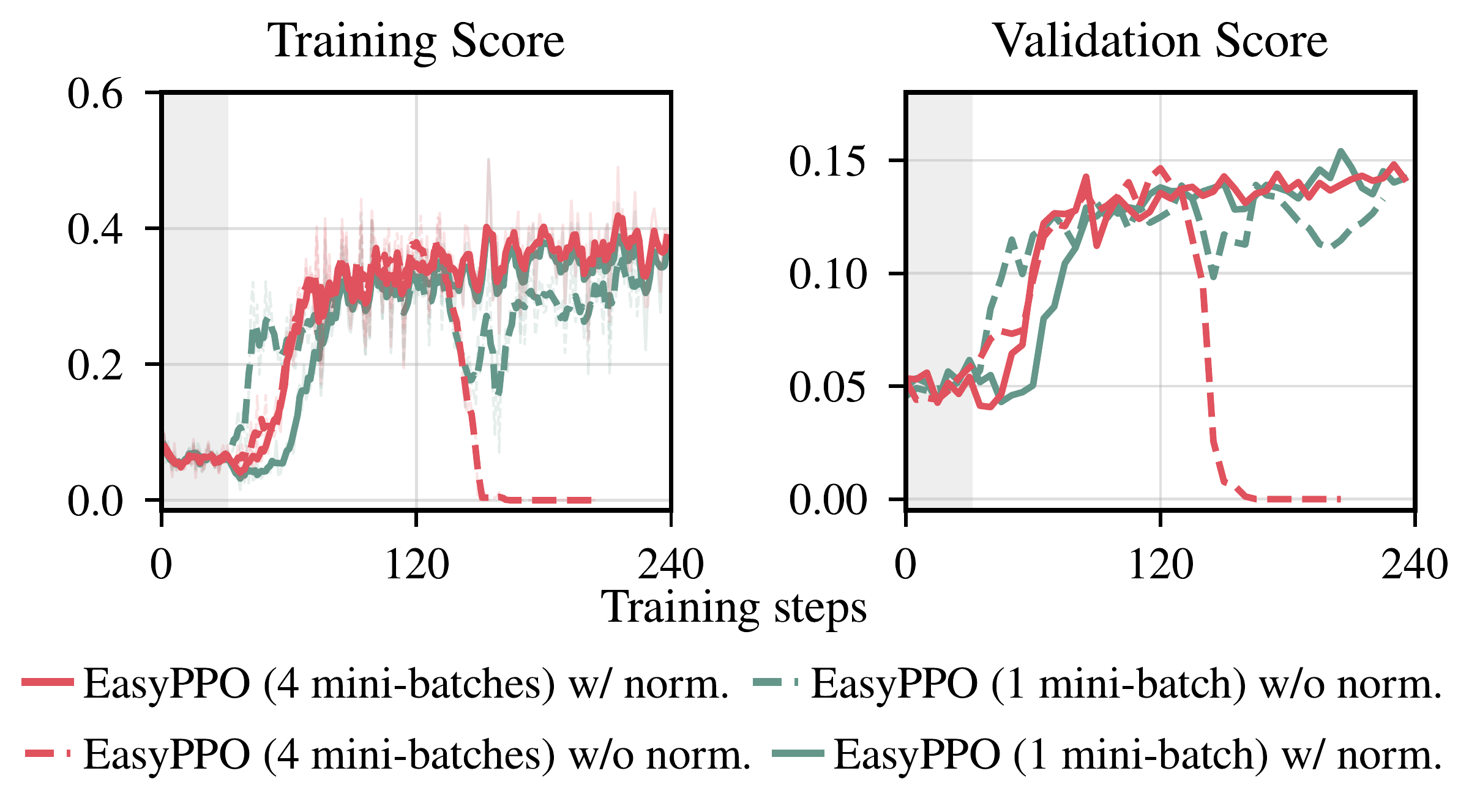
We hold the critic learning rate fixed and compare one versus four mini-batches, with and without normalization. Normalization helps both configurations. Without it, the drop with one mini-batch is recoverable, but four smaller mini-batches collapse. This matches the trade-off: splitting more finely makes return noise harder to average out.

FrontierCS training and validation scores with one or four critic mini-batches, with or without normalization. Both normalized configurations retain gains; four mini-batches without normalization collapse. — **Normalization helps both mini-batch configurations.** All runs use actor-only filtering and critic learning rate 2 × 10⁻⁶.

Does this depend on critic initialization?

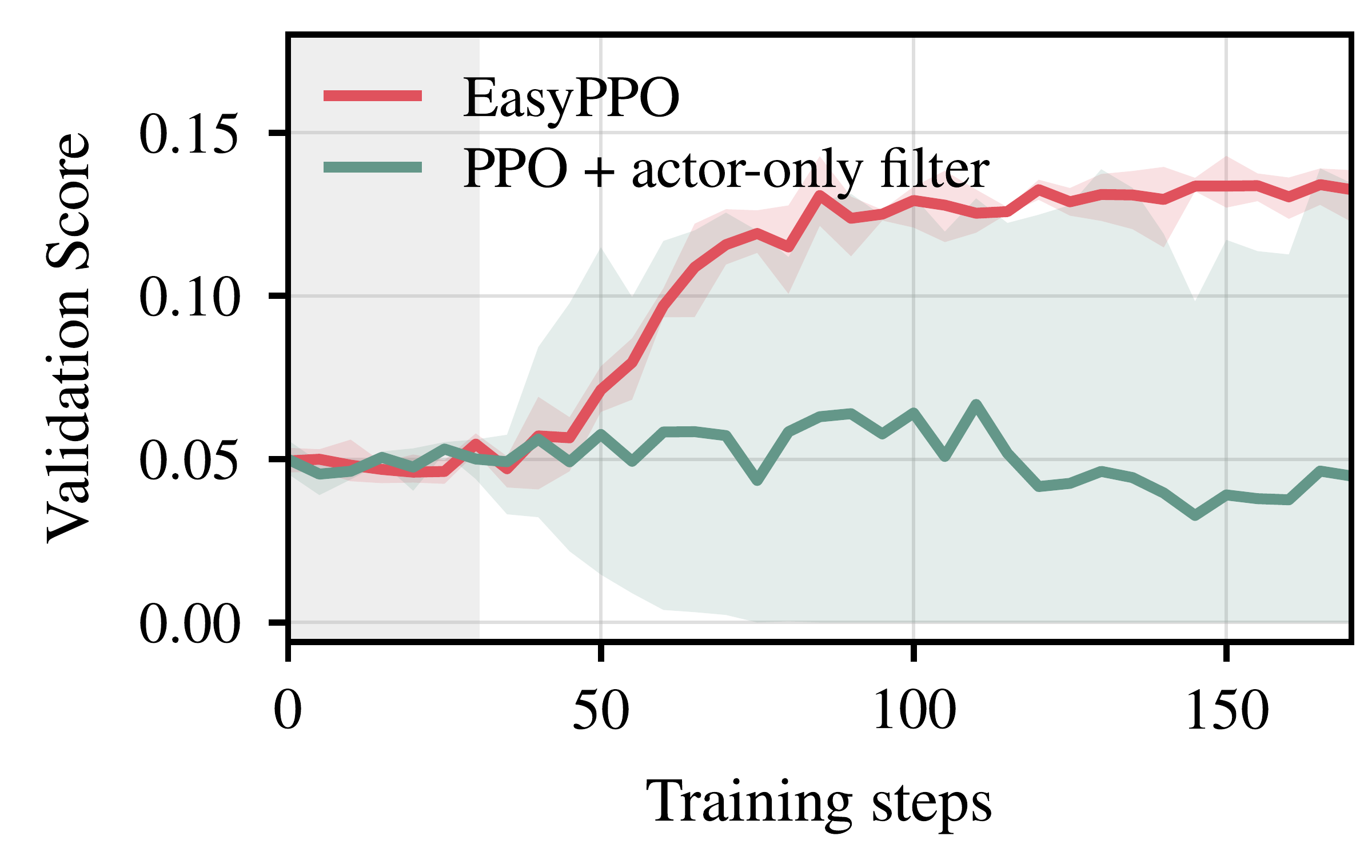
We repeat EasyPPO and PPO + actor-only filtering three times on FrontierCS, changing the critic initialization. None of the three EasyPPO runs collapses; two of the three actor-only-filtering runs do.

EasyPPO also keeps a narrow range of validation scores across runs.

Mean validation performance and minimum-to-maximum ranges across three critic initializations. EasyPPO sustains higher scores with a narrower band than PPO with actor-only filtering. — Mean and min–max range across three critic initializations per method.

The standard PPO actor can learn reliably when the critic receives complete data, balanced return noise, and updates that contain the remaining outliers.

Two rows compare critic failure modes with EasyPPO. Left: retain truncated responses for the critic only. Middle: balance gradient scales across prompts. Right: clip gradients from smaller critic mini-batches. — **Three changes to stabilize PPO through critic learning.**

References

Schulman et al. (2017). Proximal Policy Optimization Algorithms.
Li et al. (2026). When Do Larger Batches Help Scale LLM Reinforcement Learning?
Mang et al. (2025). FrontierCS: Evolving Challenges for Evolving Intelligence.
Jin et al. (2025). Search-R1: Training LLMs to Reason and Leverage Search Engines with Reinforcement Learning.
Zhou et al. (2026). Start Classifying: Categorical Critics for LLM Reinforcement Learning.
Yue et al. (2025). VAPO: Efficient and Reliable Reinforcement Learning for Advanced Reasoning Tasks.
Sheng et al. (2025). HybridFlow: A Flexible and Efficient RLHF Framework.
Qwen Team (2026). Qwen3.5: Towards Native Multimodal Agents.
He et al. (2026). FrontierSmith: Synthesizing Open-Ended Coding Problems at Scale.

BibTeX

@misc{zhou2026easyppo,
  title  = {EasyPPO: Stabilizing the Critic Is Key},
  author = {Xuanyi Zhou and Qiuyang Mang and Huanzhi Mao and
            Dacheng Li and Wenhao Chai and Mayank Mishra and Yichuan Wang and
            Karthik Narasimhan and Alvin Cheung and Joseph E. Gonzalez},
  year   = {2026},
  eprint = {2609.36802},
  archivePrefix = {arXiv},
  primaryClass  = {cs.LG},
  url    = {https://arxiv.org/abs/2609.36802}
}